Running CellART on Xenium colorectal cancer dataset
Download data
The Xenium colorectal cancer dataset can be obtained from the 10x Genomics website here, with name “Xenium In Situ, Sample P2 CRC”. Below is a demo script for create new data dir and download the required Xenium files.
[ ]:
mkdir ./xenium_crc
cd ./xenium_crc

# Download Xenium colorectal cancer dataset files
curl -O https://cf.10xgenomics.com/samples/xenium/2.0.0/Xenium_V1_Human_Colon_Cancer_P2_CRC_Add_on_FFPE/Xenium_V1_Human_Colon_Cancer_P2_CRC_Add_on_FFPE_gene_panel.json
curl -O https://cf.10xgenomics.com/samples/xenium/2.0.0/Xenium_V1_Human_Colon_Cancer_P2_CRC_Add_on_FFPE/Xenium_V1_Human_Colon_Cancer_P2_CRC_Add_on_FFPE_he_image.ome.tif
curl -O https://cf.10xgenomics.com/samples/xenium/2.0.0/Xenium_V1_Human_Colon_Cancer_P2_CRC_Add_on_FFPE/Xenium_V1_Human_Colon_Cancer_P2_CRC_Add_on_FFPE_he_imagealignment.csv
curl -O https://cf.10xgenomics.com/samples/xenium/2.0.0/Xenium_V1_Human_Colon_Cancer_P2_CRC_Add_on_FFPE/Xenium_V1_Human_Colon_Cancer_P2_CRC_Add_on_FFPE_analysis_summary.html
curl -O https://cf.10xgenomics.com/samples/xenium/2.0.0/Xenium_V1_Human_Colon_Cancer_P2_CRC_Add_on_FFPE/Xenium_V1_Human_Colon_Cancer_P2_CRC_Add_on_FFPE_outs.zip

# Unzip files
unzip Xenium_V1_Human_Colon_Cancer_P2_CRC_Add_on_FFPE_outs.zip

# Back to root dir
cd ..
The paired scRNA reference after selecting patient 2 can be download here. Please also download the reference file adata_sc_p2.h5ad into the data directory. Now you have prepared all the raw data to run CellART.
Preprocess
[ ]:
from cellart.utils.preprocess import SingleCellPreprocessor, XeniumPreprocessor
from cellart.utils.io import load_list
import scanpy as sc

# Processed data save dir
save_dir = './preprocessed_xenium_crc/'
# Transcripts and nucleus boundary files in data directory
transcripts_file = "./xenium_crc/transcripts.parquet"
nucleus_boundary_10X = "./xenium_crc/nucleus_boundaries.parquet"

st_preprocessor = XeniumPreprocessor(transcripts_file, nucleus_boundary_10X, save_dir)

# Annotated scRNA reference path
sc_adata = sc.read("./xenium_crc/adata_sc_p2.h5ad")
# Remember to specific your celltype_col and make sure your are using raw count data
sc_preprocessor = SingleCellPreprocessor(sc_adata, celltype_col = "celltype", save_path= save_dir, st_gene_list=load_list(save_dir + "/st_gene_list.txt"))

sc_preprocessor.preprocess()

st_preprocessor.prepare_sst(load_list(save_dir + "/filtered_gene_names.txt"))
st_preprocessor.get_nuclei_segmentation()
Now in the preprocessed_crc directory, you can see all the preprocessed files. You can check the spatial and segmentation files to see if their are matched.
[ ]:
# Check
import numpy as np
import matplotlib.pyplot as plt

gene_map = np.load(save_dir + "/gene_map.npy")
segmentation_mask = np.load(save_dir + "/segmentation_mask.npy")

gene_map_sum = gene_map.sum(axis=-1)
[ ]:
# plt.imshow(gene_map_sum)
# plt.imshow(segmentation_mask > 0)
fig, ax = plt.subplots(1,2, figsize=(12,5))
ax[0].imshow(gene_map_sum)
ax[0].set_title("Gene expression map sum")
ax[1].imshow(segmentation_mask > 0)
ax[1].set_title("Nuclei segmentation mask")
plt.show()
Running CellART
NOTE: these part code make takes hours to run, so it is highly recommend you not to directly run in the notebook.
[ ]:
import cellart
from pathlib import Path
import wandb
import os

# Preprocessed data
save_dir = './preprocessed_xenium_crc/'
# Directory to store all results
log_dir = "./results_xenium_crc/"

manager = cellart.ExperimentManager(
    # Basic input data settings (must be specified)
    gene_map=os.path.join(save_dir, "gene_map.npy"),
    nuclei_mask=os.path.join(save_dir, "segmentation_mask.npy"),
    basis=os.path.join(save_dir, "basis.npy"),
    gene_names=os.path.join(save_dir, "filtered_gene_names.txt"),
    celltype_names=os.path.join(save_dir, "celltype_names.txt"),
    log_dir=log_dir,

    # Training parameters (adjust based on convergence and wandb visualization)
    epochs=200,
    seg_training_epochs=10,
    deconv_warmup_epochs=100,

    pred_period=50,
    gpu="0"
)

# Update options
opt = manager.get_opt()
print(opt)
[ ]:
# Set up wandb for logging and visualization
run = wandb.init(project="CellART", dir=manager.get_log_dir(), config=opt,
                 name=os.path.basename(os.path.normpath(manager.get_log_dir())))
[ ]:
# Set up dataset
dataset = cellart.SSTDataset(manager)
gene_map_shape = dataset.gene_map.shape

# Initialize and train the CellART model
model = cellart.CellARTModel(manager, gene_map_shape, len(dataset.coords_starts))
model.train_model(dataset)
Check the output of CellART
[180]:
# Load annotated adata at epoch 200
adata = sc.read(os.path.join("./results_xenium_crc/", "epoch_200", "cell_deconv.h5ad"))
# Load segmentation
segmentation_mask = np.load(os.path.join("./results_xenium_crc/", "new_segmentation_mask.npy")).astype("int32")
[181]:
adata.obs.head()
[181]:
| x | y | celltype | |
|---|---|---|---|
| cell_id | |||
| 16712 | 383 | 1231 | Tumor III |
| 16713 | 390 | 1254 | Tumor III |
| 16714 | 385 | 1249 | Tumor III |
| 16715 | 377 | 1244 | Tumor III |
| 16716 | 384 | 1240 | Tumor III |
[182]:
segmentation_mask.shape, np.unique(segmentation_mask)
[182]:
((7271, 6669),
 array([     0,      1,      2, ..., 326938, 326939, 326940], dtype=int32))
[167]:
celltype_mapping = {
    'CAF': '#117733',  # Green
    'CD4 T cell': '#88CCEE',  # Light Blue
    'CD8 Cytotoxic T cell': '#CC6677',  # Pink
    'Endothelial': '#DDCC77',  # Sand Yellow
    'Enteric Glial': '#332288',  # Dark Blue
    'Enterocyte': '#AA4499',  # Purple
    'Epithelial': '#44AA99',  # Teal
    'Fibroblast': '#999933',  # Olive
    'Goblet': '#A1C935',  # Lime
    'Lymphatic Endothelial': '#661100',  # Brown
    'Macrophage': '#6699CC',  # Sky Blue
    'Mast': '#AA4466',  # Rose
    'Mature B': '#888888',  # Gray
    'Myofibroblast': '#117755',  # Forest Green
    'Neuroendocrine': '#332299',  # Indigo
    'Neutrophil': '#D95F02',  # Replaced duplicate pink
    'Pericytes': '#1B9E77',  # Replaced duplicate teal
    'Plasma': '#E6AB02',  # Replaced duplicate olive
    'Proliferating Immune II': '#882255',  # Burgundy
    'SM Stress Response': '#66C2A5',  # Replaced duplicate blue
    'Smooth Muscle': '#A6761D',  # Replaced duplicate brown
    'Tuft': '#7570B3',  # Replaced duplicate green
    'Tumor I': '#E7298A',  # Replaced duplicate coral
    'Tumor II': '#6A3D9A',  # Replaced duplicate navy
    'Tumor III': '#FFA500',  # Orange
    'Tumor V': '#FFD92F',  # Replaced duplicate mustard
    'Unknown III (SM)': '#B2DF8A',  # Replaced duplicate green
    'mRegDC': '#1F78B4',  # Replaced duplicate blue
    'pDC': '#8C510A',  # Replaced duplicate brown
    'vSM': '#5AB4AC',  # Replaced duplicate jade green
    "Unassigned": "lightgray",
}
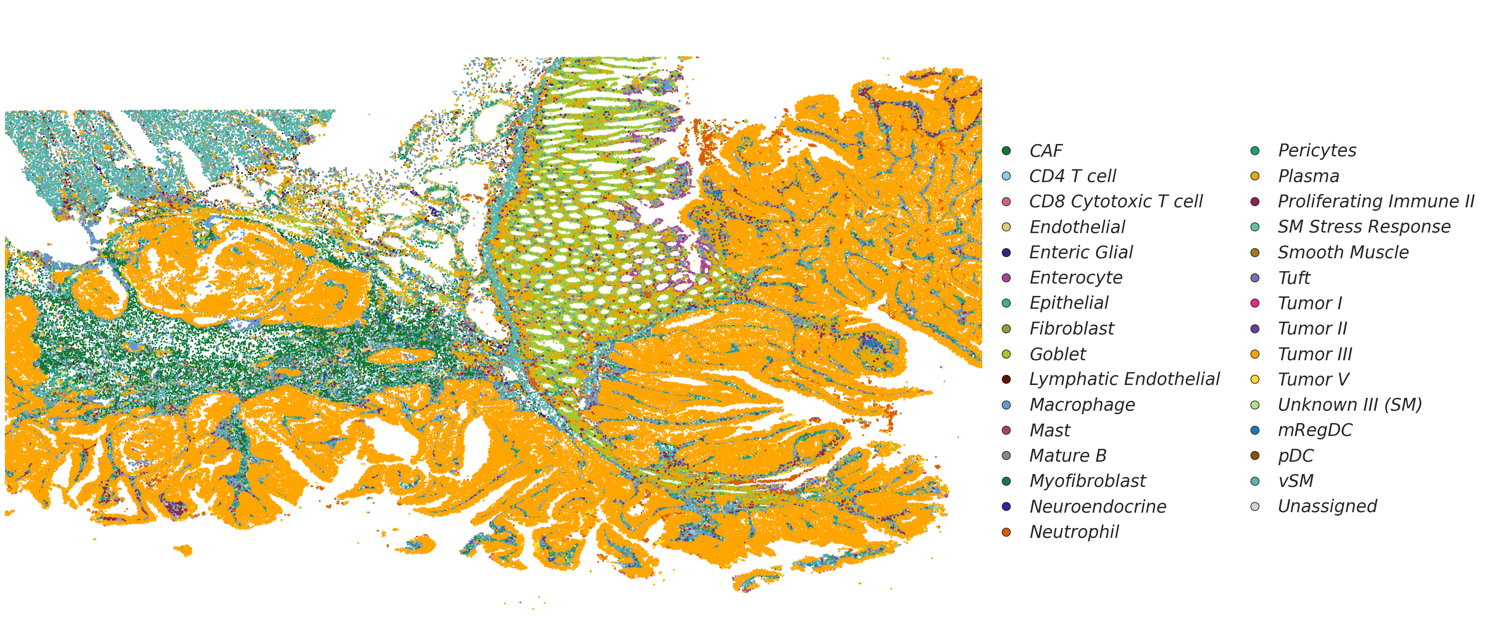
[172]:
# Visualization of cell types
from matplotlib.gridspec import GridSpec
from matplotlib.lines import Line2D
import matplotlib.pyplot as plt

fig, ax = plt.subplots(1, 4, figsize=(30, 15))
gs = GridSpec(1, 4, figure=fig)

for ax_ in ax.flatten():
    fig.delaxes(ax_)

ax1 = fig.add_subplot(gs[0, :3])
ax2 = fig.add_subplot(gs[0, 3])

celltype_names = list(celltype_mapping.keys())
# selected_celltype = ["Tumor II", "Tumor III", "Tumor V"]
selected_celltype = celltype_names
selected_celltype = celltype_names
for i in range(len(celltype_names)):
    # (0,0) is on the top left corner
    if celltype_names[i] not in selected_celltype:
        continue
    sub_df = adata[adata.obs["celltype"] == celltype_names[i - 1]].obs
    ax1.scatter(sub_df["x"], sub_df["y"], s=3, label=celltype_names[i - 1], color=celltype_mapping[celltype_names[i - 1]])
# ax1.invert_yaxis()
ax1.axis("off")
ax1.set_xlim(adata.obs["y"].min(), adata.obs["y"].max())
ax1.set_ylim(adata.obs["x"].min(), adata.obs["x"].max())
ax1.invert_xaxis()

# Add legend elements (example)
legend_elements = [
    Line2D(
        [0], [0],
        marker='o',
        linestyle='None',
        color='w',
        label=label,
        markerfacecolor=color,
        markeredgecolor='k',
        markersize=12
    ) for label, color in celltype_mapping.items()
]

# Add the legend below the entire figure, centered horizontally with [0, 1] subfigures
ax2.legend(
    handles=legend_elements,
    loc='center',                    # Center the legend within the bounding box
    bbox_to_anchor=(0.48, 0.45),       # Center of ax2 (0.5, 0.5 is the middle of the axis)
    ncol=2,                          # Number of columns for the legend
    handletextpad=0.35,               # Spacing between marker and text
    columnspacing=1,               # Spacing between legend columns
    prop={'size': 25, 'style': 'italic'},  # Font size and style
    frameon=False                    # No border for the legend
)

ax2.axis("off")  # Hide the axis for ax2
# Adjust layout to prevent overlap
plt.tight_layout(rect=[0, 0.15, 1, 1])  # Leave space for the legend below the plots
plt.show()
Visualize segmentation and annotation through SpatialData
[183]:
from cellart.utils.spatialdata_utils import append_xenium_boundary
from spatialdata_io import xenium
import spatialdata_plot

sdata = xenium("./xenium_crc/", aligned_images=False)
INFO reading /import/home3/yhchenmath/Dataset/DeconvSeg/CRC/Xenium_P2_CRC/cell_feature_matrix.h5
[184]:
# Append cellart results to SpatialData
append_xenium_boundary(segmentation_mask, sdata, "cellart_boundaries", celltype = adata.obs["celltype"])
[185]:
# Select a region of interest (ROI) for visualization
x_min, x_max, y_min, y_max = 13000, 17000, 5500, 9500
sdata_roi = sdata.query.bounding_box(
    min_coordinate=[x_min, y_min], max_coordinate=[x_max, y_max], axes=("y", "x"), target_coordinate_system="global"
)
[186]:
for k in ["cellart_boundaries"]:
    ct_col = sdata_roi.shapes[k].celltype
    cts = sdata_roi.shapes[k].celltype.unique()
    for ct in cts:
        sdata_roi.shapes[f"{k}_{ct.replace(' ', '_').replace('(', '').replace(')', '')}"] = \
        sdata_roi.shapes[k][ct_col == ct]
[190]:
def plot_annotation(sdata, shape_key, ax):
    tmp = None
    draw_cts = sdata.shapes[shape_key].celltype.unique().tolist()
    for ct in draw_cts:

        color = celltype_mapping[ct]
        if tmp is None:
            tmp = sdata.pl.render_shapes(
            f"{shape_key}_{ct.replace(' ', '_').replace('(', '').replace(')', '')}",
            color=color, fill_alpha=0.45, outline_width=0.5, outline_alpha=1, outline_color = color
            )
        else:
            tmp = tmp.pl.render_shapes(
                f"{shape_key}_{ct.replace(' ', '_').replace('(', '').replace(')', '')}",
                color=color, fill_alpha=0.6, outline_width=1, outline_alpha=1, outline_color = color
            )
    tmp.pl.show(coordinate_systems="global", ax=ax, title="", frameon=False, legend_loc='none', colorbar=False)
    ax.axis('off')
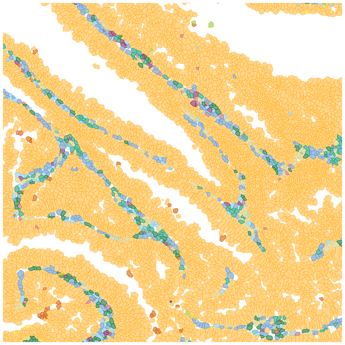
[191]:
fig, ax = plt.subplots(1, 1, figsize=(15,15))

plot_annotation(sdata_roi, "cellart_boundaries", ax)

ax.set_xlim(y_min, y_max)
ax.set_ylim(x_min, x_max)
plt.show()
INFO     Value for parameter 'color' appears to be a color, using it as such.
INFO     Value for parameter 'color' appears to be a color, using it as such.
INFO     Value for parameter 'color' appears to be a color, using it as such.
INFO     Value for parameter 'color' appears to be a color, using it as such.
INFO     Value for parameter 'color' appears to be a color, using it as such.
INFO     Value for parameter 'color' appears to be a color, using it as such.
INFO     Value for parameter 'color' appears to be a color, using it as such.
INFO     Value for parameter 'color' appears to be a color, using it as such.
INFO     Value for parameter 'color' appears to be a color, using it as such.
INFO     Value for parameter 'color' appears to be a color, using it as such.
INFO     Value for parameter 'color' appears to be a color, using it as such.
INFO     Value for parameter 'color' appears to be a color, using it as such.
INFO     Value for parameter 'color' appears to be a color, using it as such.
INFO     Value for parameter 'color' appears to be a color, using it as such.
INFO     Value for parameter 'color' appears to be a color, using it as such.
INFO     Value for parameter 'color' appears to be a color, using it as such.
INFO     Value for parameter 'color' appears to be a color, using it as such.